18. 12. 2024 Charles Callaway Documentation

Explaining Your Content with Complex Animations, Part 2

Hi again! At the end of my last blog I left you hanging. I promised some concrete examples of useful animations you could do in-house, using just math. And here I am, examples in hand!

Although they could be finished animations in specific situations, they’re more likely to be parts of a larger picture, so it’s more important to see how they’re made so you can understand them and then adapt them to your needs. We’ll look at:

A sunset where the sun sinks below the horizon
A histogram that looks the equalizer on a stereo
Just in time for December, falling snow

Before we start with my 3 animations though, let’s take a quick look at how you can get some ideas. After all, there are tons of static 2D matplotlib examples out there and very few animations. What do you need to do to convert one into the other?

Going from Static to Dynamic

The “Hello World” example in MatPlotLib/Python is the sine wave. So let’s see what the static and animated version look like side-by-side:

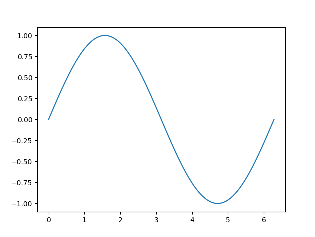
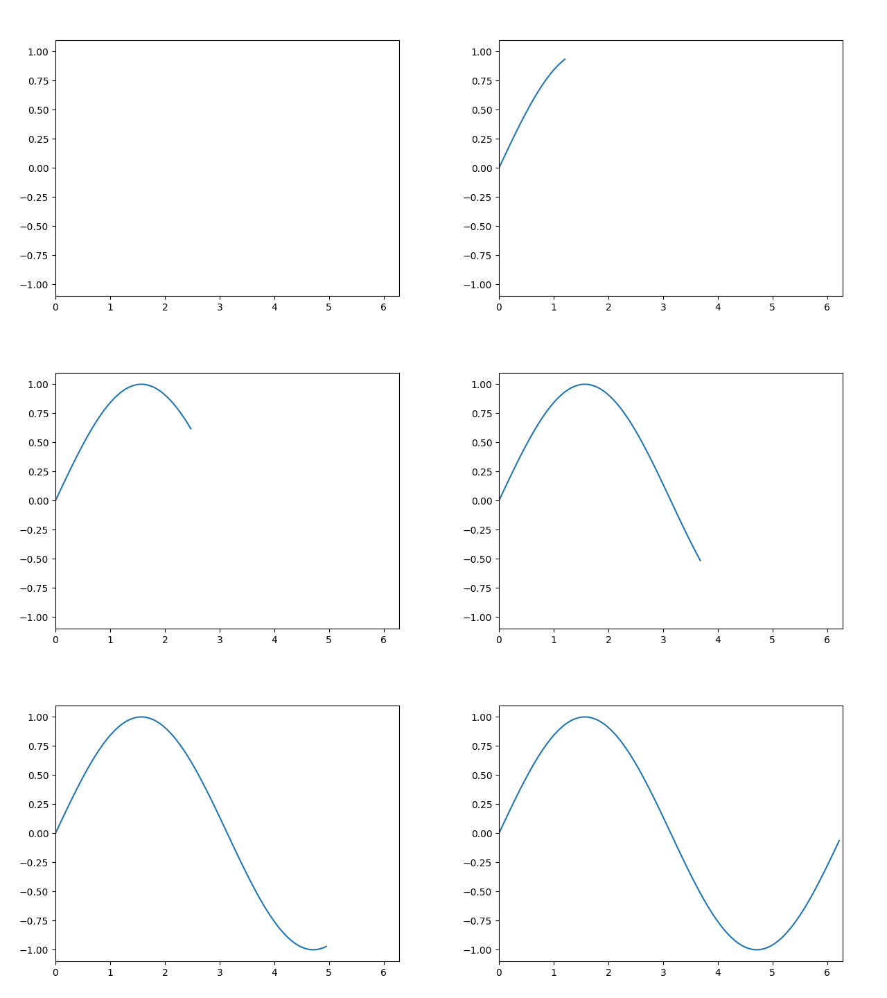
To run one of them, open the command prompt in the directory where you saved the file, and then run python sine.py (or whatever name you gave the file, and assuming you’ve already installed Python).

import matplotlib.pyplot as plt
import matplotlib.animation as animation
import numpy as np

X = np.linspace(0, 2*np.pi, 100)
Y = np.sin(X)

plt.plot(X,Y)
plt.show()

import matplotlib.pyplot as plt
import matplotlib.animation as animation
import numpy as np

X = np.linspace(0, 2*np.pi, 100)
Y = np.sin(X)

fig, ax = plt.subplots(1,1)
ax.set_xlim([0, 2*np.pi])
ax.set_ylim([-1.1, 1.1])
sinegraph, = ax.plot([], [])

def update(i):
    sinegraph.set_data(X[:i],Y[:i])

anim = animation.FuncAnimation(fig, update,
                    frames=len(X), interval=50)
plt.show()

You can see that most of the additions have to with animation stuff: setting up the camera viewport and specifying what data to show when.

The static code on the left consists of:

Imports (lines 1-3)
Setting up the data (lines 5-6)
Plot the computed data and show it (pops up a static screen) (lines 8-9)

The animation code has both similarities and differences:

Imports (lines 1-3)
Setting up the data (lines 5-6)
Lay out the graphic elements (lines 8-11; you could do this in the static version but I used the defaults)
Create an animation “update” function called for at each frame (lines 13-14) (updating both data to draw and graphic elements)
Draw the frames of the plot, saving them to a file (lines 16-18)

For the last point you basically need to know how many frames per second you want, how many frames total, and whether to show it immediately or save it as a file (and thus any animation options needed by the animation program).

If you replace the very last line in the animation version above with this, you can save it as an animated GIF or video file (file format determined by filename extension):

anim.save('sine-wave.gif', fps=10)

Sunset Time!

With that out of the way, let’s look at our first video-worthy example. We’ll create a full-screen animation of a yellow sun on an orange background as it slowly sets:

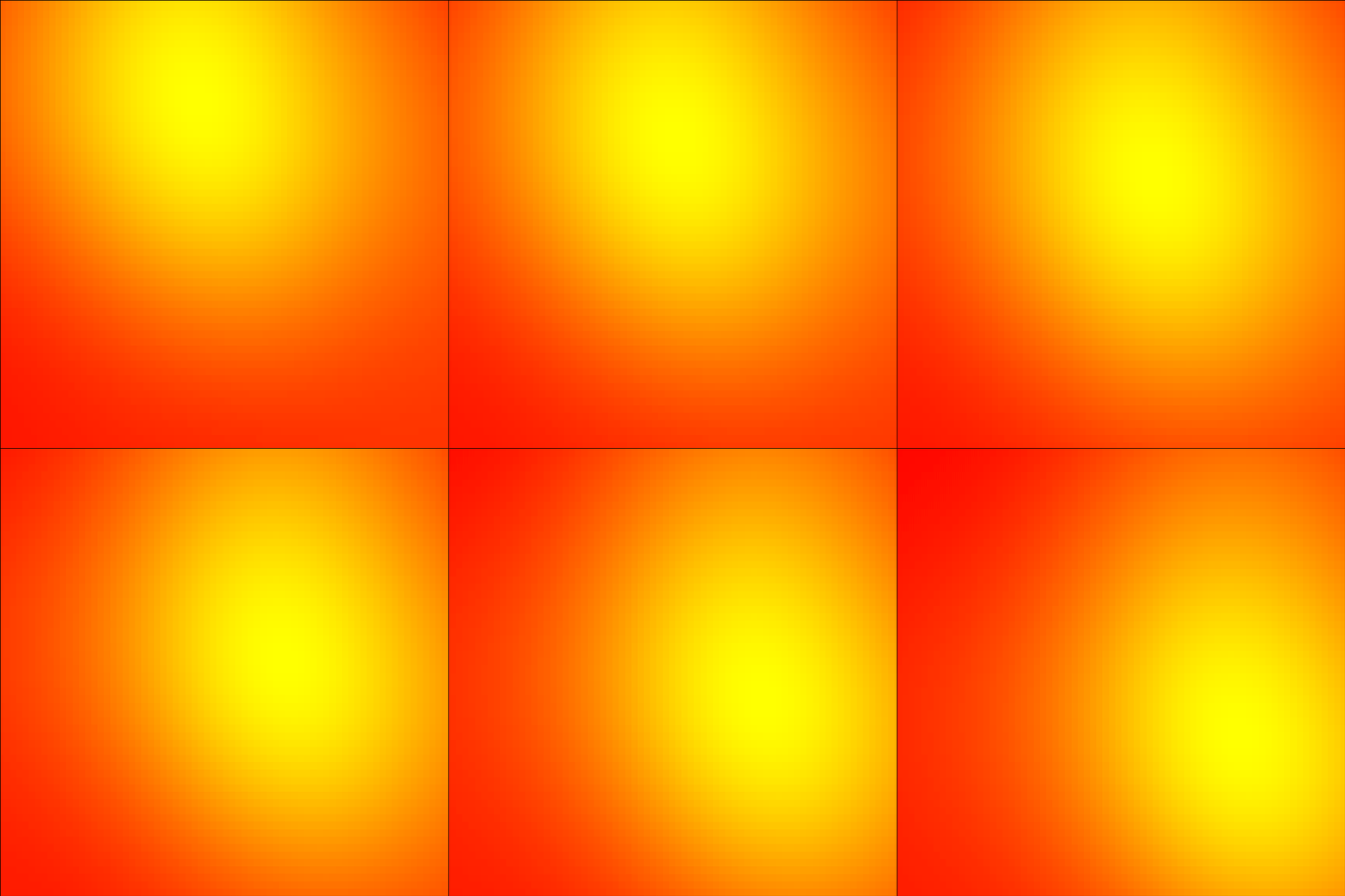
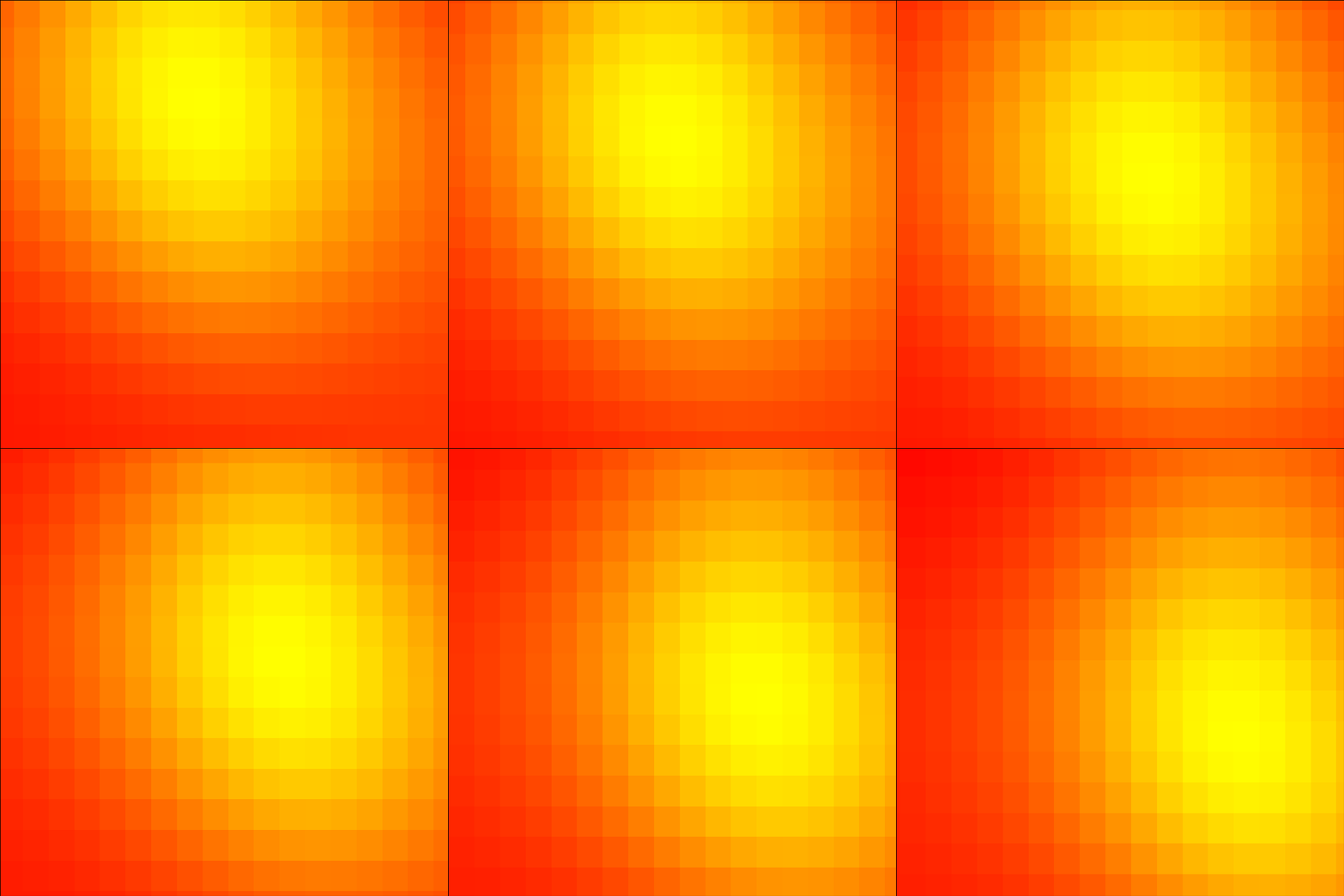
Here we can assume that because it fills up a rectangle, it’ll be either full-screen or set in some kind of rectangular frame within a larger video (there are other options that involve transparency).

If we look at the code, it’s more complicated, but it still has the same basic parts. Changing parameters like the pixel size (try changing nbins in line 16 from 120 to 300) is easy because it’s just math. In fact what’s typically most complicated is the creation and organization of the data (lines 7-24) and the animation frame updates (lines 26-32).

The animation update function tells us how the animation works: the “sunset” plot is actually much larger than the visible area on the screen, and frame updates basically “pan” across the yellow spot, moving the frame slowly up and leftward so it appears the “sun” is slowly moving down. In fact it’s just like standard cinematography.

import pandas as pd
import matplotlib.pyplot as plt
import numpy as np
import matplotlib.animation as animation
from scipy.stats import gaussian_kde

global df, xi, yi, zi, nbins

np.random.seed(411)
df = pd.DataFrame({
       'x': np.random.vonmises(.2, .8, size=20),
       'y': np.random.vonmises(.9, .7, size=20)
     })
df.head()
# Init values and parameters
nbins = 120
x = df['x'] # change 'x' with your column name
y = df['y'] # change 'y' with your column name
k = gaussian_kde([x,y])
xi, yi = np.mgrid[
         x.min():x.max():nbins*1j,
         y.min():y.max():nbins*1j    ]
zi = k(np.vstack([xi.flatten(),
                  yi.flatten()] )).reshape(xi.shape)

def update(frame):
    ax.clear()
    # real limits: -2.3<-->2.5
    ax.set_ylim(-1.5+frame/80, 1.5+frame/80)
    ax.set_xlim(-0.8-frame/110, 2.0-frame/110)
    ax.pcolormesh(xi, yi, zi, cmap='autumn')
    return fig,

fig, ax = plt.subplots(figsize=(8,8))
ax=fig.add_axes([0,0,1,1])
ax.set_axis_off()
ani = animation.FuncAnimation(fig, update, frames=range(0, 100))
ani.save('sunset.gif', fps=10)

Musical Histogram

It’s important to remember that a video isn’t just all graphics. There’s also music and sound effects. And sometimes you want to make them reinforce each other. So why not a playful equalizer that moves in time with the music? Yes, you can do that with math (well, the synchronization isn’t included here…)

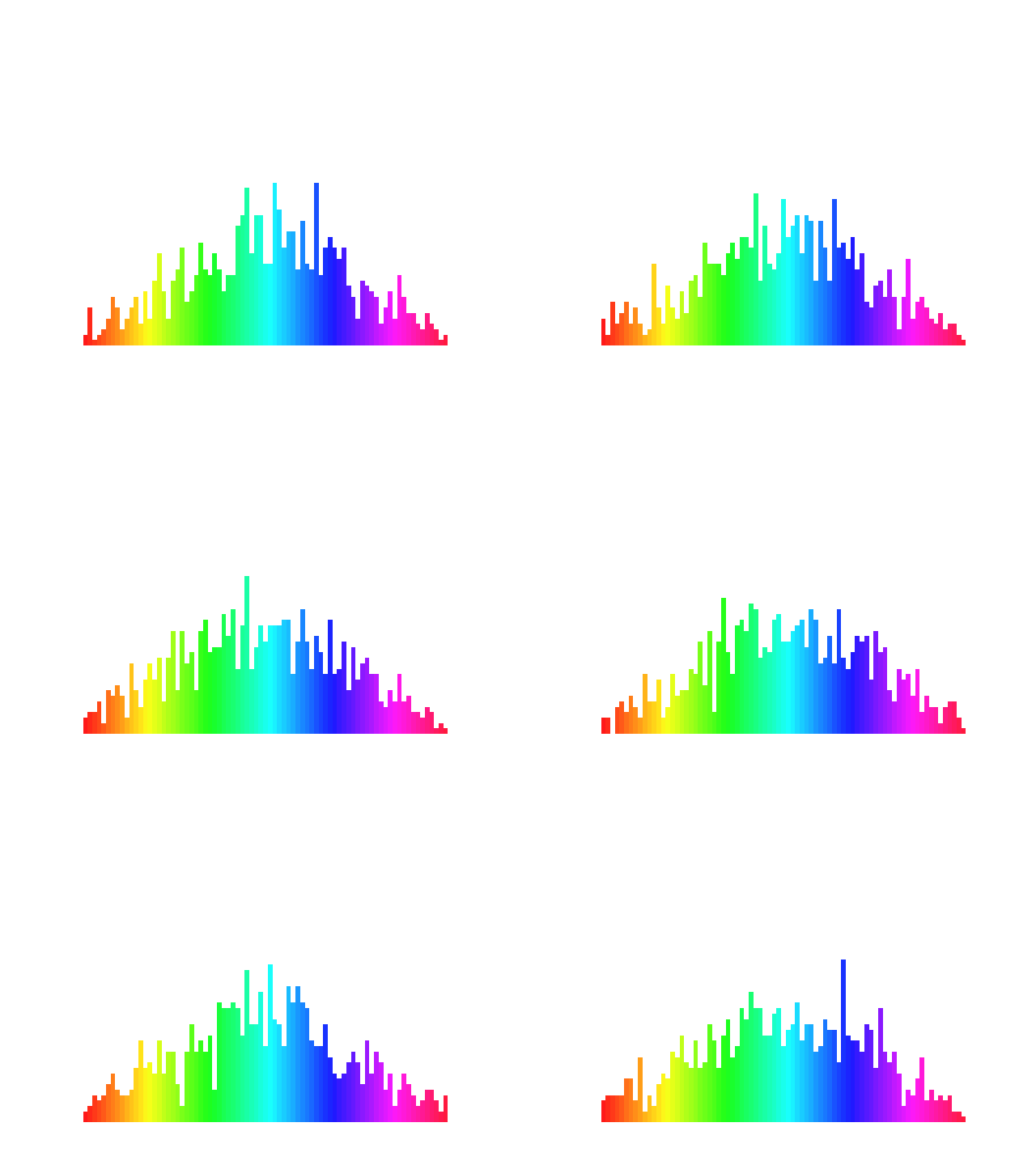
This animation takes advantage of the built-in colormap feature, which means we don’t have to assign colors between each animation frame, just the column heights.

Again you’ll notice the structure of the code is basically the same. What we’ve changed is the graph type and the mathematical approach (although they’re both based on statistical distributions).

Unlike the panning approach of the frame’s viewport with the sunset above, here it stays where it is and we draw the rectangles of the bar graph, then erase and draw them again with the new values at the beginning of the next frame.

import functools
import matplotlib.pyplot as plt
import numpy as np
import matplotlib.animation as animation

# Setting up a random number generator with a fixed state for reproducibility.
rng = np.random.default_rng(seed=83801)
# Fixing bin edges.
HIST_BINS = np.linspace(-2, 2, 80)

# Histogram our data with numpy.
data = rng.standard_normal(1000)
n, _ = np.histogram(data, HIST_BINS)

cm = plt.colormaps.get_cmap('hsv')

def animate(frame_number, bar_container):
    data = rng.standard_normal(1000)
    n, _ = np.histogram(data, HIST_BINS)
    # scale values to interval [0,1]
    col = HIST_BINS - min(HIST_BINS)
    col /= max(col)
    for count, c, rect in zip(n, col, bar_container.patches):
        rect.set_height(count)
        plt.setp(rect, 'facecolor', cm(c))
    return bar_container.patches

fig, ax = plt.subplots()
_, _, bar_container = ax.hist(data, HIST_BINS, lw=1, alpha=0.9)
ax.set_ylim(top=55)  # set safe limit to ensure that all data is visible.
ax.set_axis_off()

anim = functools.partial(animate, bar_container=bar_container)
ani = animation.FuncAnimation(fig, anim, 50, repeat=False, blit=True)
ani.save('histogram.gif', fps=10)

Snowflakes

While I’m writing this it’s mid-December, so how about we create a wintry animation, something like snowflakes gently falling from the sky? We’ll use randomized arrays to really start ratcheting up the number of individual elements we’re animating. One dimension will be the element, and the other dimension will be its properties.

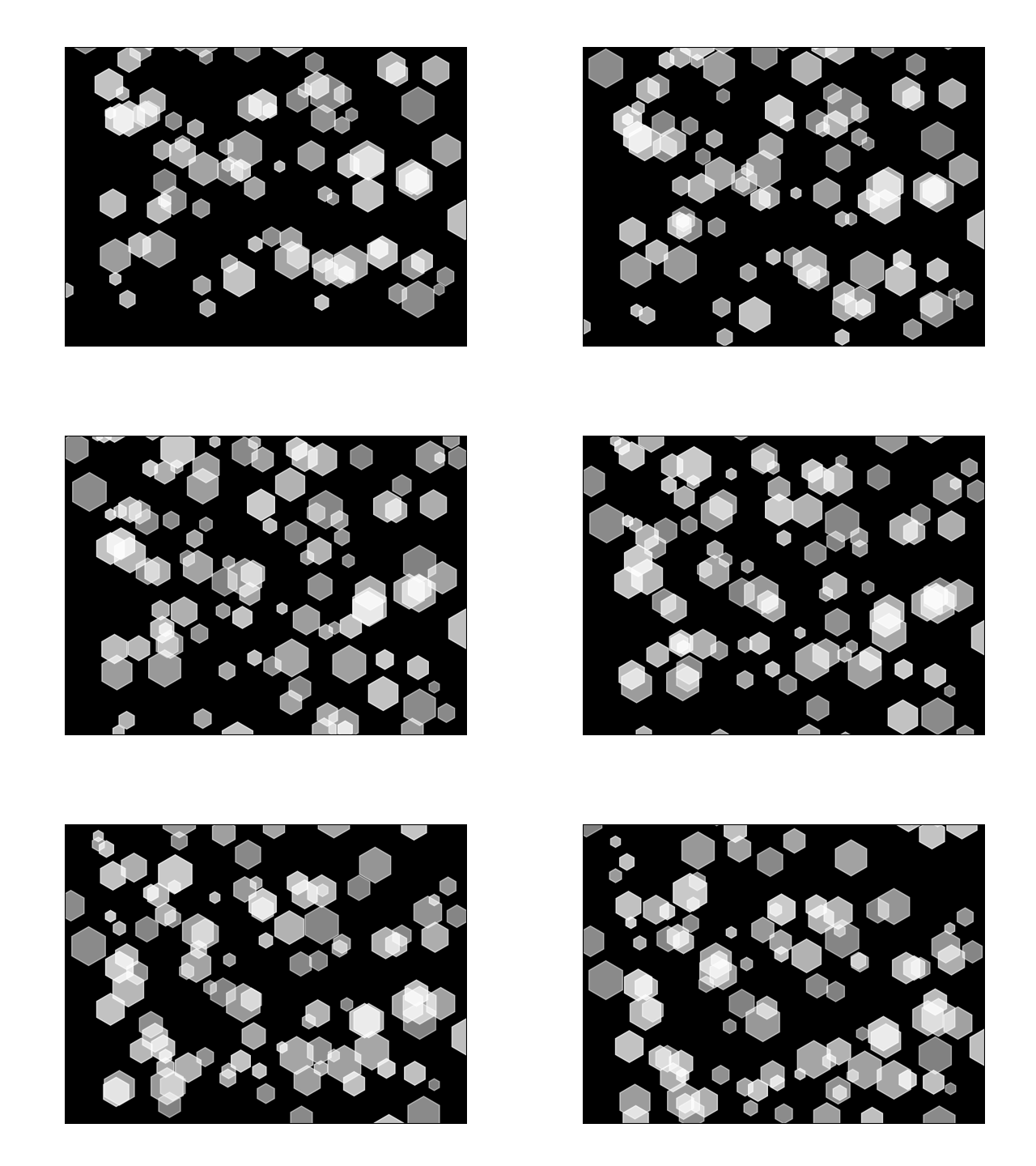
In this example we’ll do a different version of panning. The viewport will stay at [0..1,0..1] and we’ll put the snowflakes initially both in and far above the viewport, giving each one a falling speed, a width, and alpha transparency (all random within set ranges). Then during the frame update loop we’ll always lower their Y values by that speed, give them a bit of horizontal jiggle, and when the animation is over, they’ll still be falling, but new ones will arrive from above.

And as before, we still have the basic structure: data, graph setup, and frame-by-frame animation. Most of the graph setup is to get rid of the axes and the area immediately surrounding the graph where the axes had been. Other than that, it’s the typical “figure out the math” and then you’re off to making some small tweaks to make it video-ready.

import matplotlib.pyplot as plt
import pandas as pd
import numpy as np
import matplotlib.animation as animation

rng = np.random.default_rng(seed=8398201)
n = 400                 # Number of snowflakes
fps = 10                # Frames per second
length = 6              # How long animation lasts, in seconds
r = np.random.rand(n,5) # <n> snowflakes, 4 random values: x,y,speed,size,alpha
r[:,0] *= 1.4           # Scale a bit left and right so some appear partway off screen
r[:,0] += -0.2          # Should now have values [-0.2..1.2]
r[:,1] *= 6             # Scale the initial vertical distribution upwards so they keep falling
r[:,2] *= 0.015         # Standard downward speed
r[:,2] += np.random.random()*0.005  # Some faster, some slower:  [0.020..0.015] per frame
r[:,3] *= 25
r[:,3] += 10            # Each snowflake size = [0..1]*25+10 = [10..25]
r[:,4] *= 0.3
r[:,4] += 0.5           # Set the alpha from [0.5..0.8]

def update(frame):
    ax.clear()             # Wipe the previous data points
    ax.set_xlim(-0.2,1.2)  # Fix the axes
    ax.set_ylim(-0.2,1.2)
    # For this frame, draw all its snowflakes
    for i in range(0, n):
      r[i,0] = r[i,0]+(0.003-0.006*np.random.random())  # Move a snowflake a bit left or right
      r[i,1] = r[i,1]-r[i,2]   # Move the snowflake down at its own speed
      # Plot the snowflake, using a white hexagon
      ax.plot(r[i,0], r[i,1], marker='h', markersize=r[i,3], color='white', alpha=r[i,4])
    return fig,

fig, ax = plt.subplots()           # Create the graph
ax.get_xaxis().set_visible(False)  # Don't show the axes
ax.get_yaxis().set_visible(False)
ax.set_facecolor('#000000')        # Set the background color to black
fig.patch.set_visible(False)       # Make the margins smaller

# Iterate through all *n* frames, drawing them one by one, and saving them as an animated GIF
ani = animation.FuncAnimation(fig, update, frames=range(0, length*fps), repeat=True)
ani.save('snow.gif', fps=fps)  # Animation length in seconds is #frames/fps

Conclusion

So there are three real-world examples you can use and build on to create animations as part of your videos. Of course, further work will be necessary to customize them (size, aspect ratio, colors, length, etc.) and improve the quality.

Unlike a manual approach like I described with PowerPoint in my last blog post though, we can animate hundreds or thousands of distinct elements without having to do them one by one. If we can describe it in math, we can show it and animate it. And we can usually tweak parameters just by changing a few numbers or formulas.

There’s one thing missing so far with the animated GIFs we create: there’s no transparency. This isn’t a problem with the sunset example since it’s intended to be a background, but we’d really like to put our equalizer or snowflakes somewhere in the foreground. And that means they need a transparent background. But I’m sure you can wait until my next post. 😜